Complete Guide: Installing CUDA and Verifying PyTorch Installation

How to install CUDA+Pytorch to run my FIRST machine learning code on MY OWN computer?

First, install CUDA:

Install CUDA Toolkit

In my case I downloaded it from

Chose the right version for you.

In my case, I choose the options shown below:

Options for Ubuntu 20, and runfile (local)

After selecting the options that fit your computer, at the bottom of the page we get the commands that we need to run from the terminal. In my case, I executed the following in the terminal:

wget https://developer.download.nvidia.com/compute/cuda/12.1.0/local_installers/cuda_12.1.0_530.30.02_linux.runsudo 
sh cuda_12.1.0_530.30.02_linux.run

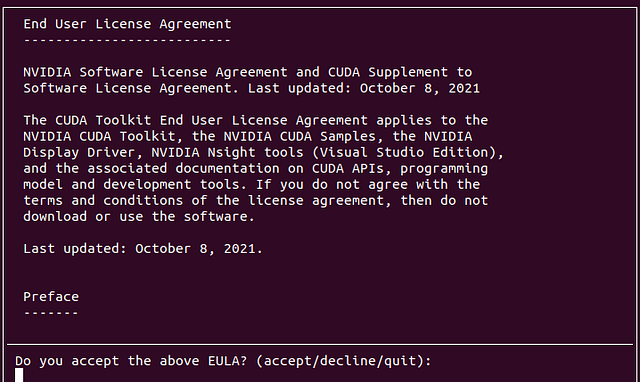
Proceed with the installation

You should see the following sequence of screens

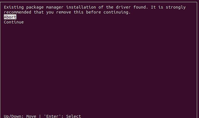
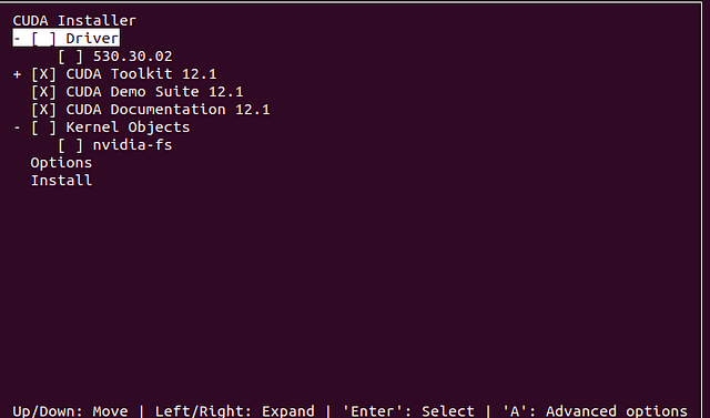
I would try without installing the driver first.

Note that I did not choose to install the Driver!

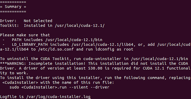
If the installation was successful, you will see something similar to

Installing Pytorch

Go to https://pytorch.org/get-started/locally/

You will be presented these screen (at the time of writing this post, this is what we see)

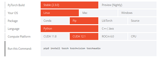
MAKE sure that you select the CUDA version that you installed in the previous step. In my case I installed CUDA 12.1 in the previous step, so I select CUDA12.1 when installing Pytorch. Run the command that appears at the bottom. In my case, you see that I need to run the following:




pip3 install torch torchvision torchaudio

I executed this command in the terminal.

While the installation was taking place I got this error:

ERROR: Package ‘networkx’ requires a different Python: 3.8.10 not in ‘>=3.9’

So I installed a different networkx package that is supported with my current system setup. To install the different (slighly older) networkx package, I executed the following in the terminal:

pip install networkx==3.1

Then I tried the installation again with

pip3 install torch torchvision torchaudio --index-url https://download.pytorch.org/whl/cu118

This time all worked!

Verifying installation

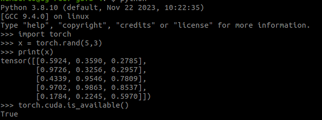
To verify the Pytorch install, we can run the following in the terminal. First start a Python session by typing “python” in the terminal. You should see something similar to

Python 3.8.10 (default, Nov 22 2023, 10:22:35) 
[GCC 9.4.0] on linux
Type "help", "copyright", "credits" or "license" for more information.python

Then execute the following

import torch
x = torch.rand(5, 3)
print(x)

The output should be similar to

tensor([[0.5924, 0.3590, 0.2785],
        [0.9726, 0.3256, 0.2957],
        [0.4339, 0.9546, 0.7809],
        [0.9702, 0.9863, 0.8537],
        [0.1784, 0.2245, 0.5970]])

Now, to check if CUDA is available, do

import torch
torch.cuda.is_available()

If CUDA is there you should see “True” in the terminal.

Altogether the verification steps in my terminal look like the following:

At this point you should be able to run a machine learning application locally.

Now the fun part. Try the following code:

# Importing necessary libraries
import torch
import torch.nn as nn
import torch.optim as optim
import numpy as np
from sklearn.datasets import load_iris
from sklearn.model_selection import train_test_split
from sklearn.preprocessing import StandardScaler
from sklearn.metrics import accuracy_score, confusion_matrix
import matplotlib.pyplot as plt
import seaborn as sns

# Setting random seed for reproducibility
torch.manual_seed(42)

# Loading the Iris dataset
iris = load_iris()
X, y = iris.data, iris.target

# Splitting the data into training and testing sets
X_train, X_test, y_train, y_test = train_test_split(X, y, test_size=0.2, random_state=42)

# Standardizing the features
scaler = StandardScaler()
X_train = scaler.fit_transform(X_train)
X_test = scaler.transform(X_test)

# Convert NumPy arrays to PyTorch tensors
X_train = torch.tensor(X_train, dtype=torch.float32)
X_test = torch.tensor(X_test, dtype=torch.float32)
y_train = torch.tensor(y_train, dtype=torch.long)
y_test = torch.tensor(y_test, dtype=torch.long)

# Define a simple neural network model
class SimpleNN(nn.Module):
    def __init__(self, input_size, hidden_size, num_classes):
        super(SimpleNN, self).__init__()
        self.fc1 = nn.Linear(input_size, hidden_size)
        self.relu = nn.ReLU()
        self.fc2 = nn.Linear(hidden_size, num_classes)

    def forward(self, x):
        out = self.fc1(x)
        out = self.relu(out)
        out = self.fc2(out)
        return out

# Parameters
input_size = X_train.shape[1]
hidden_size = 128
num_classes = len(np.unique(y_train))
num_epochs = 100
learning_rate = 0.001

# Initialize the model
model = SimpleNN(input_size, hidden_size, num_classes)

# Loss and optimizer
criterion = nn.CrossEntropyLoss()
optimizer = optim.Adam(model.parameters(), lr=learning_rate)

# Lists to store the training loss over epochs
train_losses = []

# Training the model
for epoch in range(num_epochs):
    # Forward pass
    outputs = model(X_train)
    loss = criterion(outputs, y_train)

    # Backward pass and optimization
    optimizer.zero_grad()
    loss.backward()
    optimizer.step()

    train_losses.append(loss.item())

    if (epoch+1) % 10 == 0:
        print(f'Epoch [{epoch+1}/{num_epochs}], Loss: {loss.item():.4f}')

# Plotting the training loss over epochs
plt.plot(train_losses, label='Training Loss')
plt.xlabel('Epoch')
plt.ylabel('Loss')
plt.title('Training Loss Over Epochs')
plt.legend()
plt.show()

# Evaluating the model
with torch.no_grad():
    outputs = model(X_test)
    _, predicted = torch.max(outputs, 1)
    accuracy = accuracy_score(y_test.numpy(), predicted.numpy())
    print('Accuracy:', accuracy)

    # Creating a confusion matrix
    cm = confusion_matrix(y_test.numpy(), predicted.numpy())
    plt.figure(figsize=(8, 6))
    sns.heatmap(cm, annot=True, fmt='d', cmap='Blues', xticklabels=iris.target_names, yticklabels=iris.target_names)
    plt.xlabel('Predicted')
    plt.ylabel('True')
    plt.title('Confusion Matrix')
    plt.show()

The expected outcome of this algorithm is a trained neural network model that can accurately classify instances of the Iris dataset into one of the three classes (Setosa, Versicolor, or Virginica).

After training, the model is evaluated on the testing set to assess its performance on unseen data. The evaluation metric used in this example is accuracy, which measures the proportion of correctly classified instances in the testing set.

After running this example you will see the following plots:

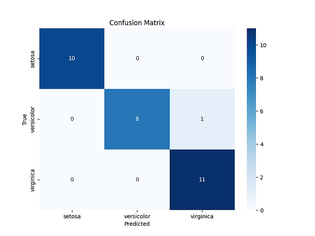
This confusion matrix shows that for the code above, the network predicts the classes accurately, except for one example (the cell with the number 1). This number 1 in the cell (2,3) means that for one of the examples, the neural network predicted that the class was Virginica but the correct class was Versicolor.

Overall, the neural network only made one mistake.

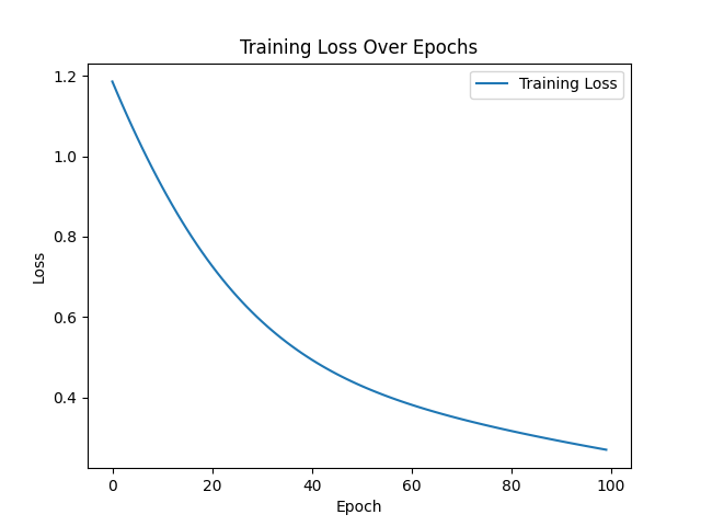
This last plot simply shows that as the neural goes over the examples, the training is gradually having better predictions (lower cost, better network responses-not generally, but for the purposes of this article we can settle here).

Good luck!