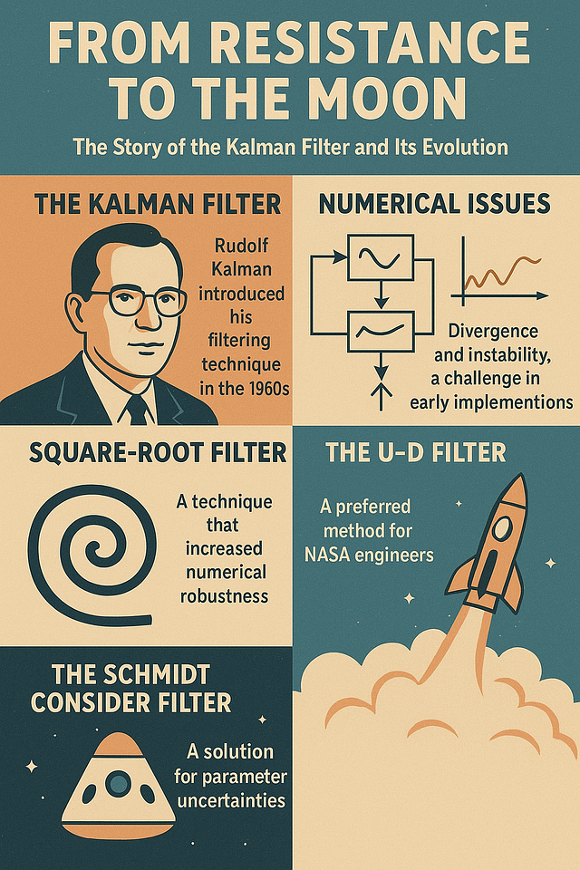
When Rudolf Kalman introduced his filtering technique in the 1960s, it wasn’t immediately embraced. In fact, the reception was so chilly that he ended up publishing his groundbreaking work in a mechanical engineering journal — rather than in electrical engineering, where one might have expected it. Many of his peers simply weren’t convinced.

But Kalman persisted. His insistence on sharing his ideas eventually caught the attention of researchers in other fields. Among them: NASA engineers. By the fall of 1960, Kalman visited NASA’s Ames Research Center, where he met Stanley Schmidt from the Dynamics Analysis Branch. Schmidt’s team was wrestling with midcourse navigation for the Apollo missions, constrained by the limited onboard computers of the time.

Schmidt immediately saw potential in Kalman’s approach. While the filter had been designed for linear systems, Schmidt realized it could be adapted for nonlinear cases by linearizing around a reference trajectory. NASA engineers soon improved on this idea: instead of linearizing around a reference, they would linearize around the current estimate generated by the filter itself.

Thanks to collaborations with colleagues like Richard Battin at MIT’s Instrumentation Laboratory, Schmidt helped push the Kalman filter into the heart of Apollo’s guidance and navigation system. Still, before it could fly astronauts to the Moon, engineers had to confront some serious numerical problems.

Cracks Beneath the Surface: Numerical Issues

The Kalman filter’s popularity soared after its success in Apollo midcourse navigation. But real-world implementations quickly exposed a dark side: divergence and instability.

NASA studies combining radar data with onboard sensors revealed that, under certain conditions, the filter could blow up. Early on, these problems were blamed on the limitations of 16-bit computers. But it became clear that the very structure of the Kalman equations — particularly the covariance update step, which subtracts two positive-definite matrices — was also vulnerable to numerical errors.

Engineers responded with clever ad-hoc fixes. They enforced matrix symmetry by averaging terms, clipped correlation coefficients above one, or even added small numbers to diagonal terms (a trick known as covariance inflation). While these hacks worked, they felt more like patch jobs than principled solutions. Decades later, mathematics would validate that these were, in fact, sound techniques.

---

Enter Square-Root Filtering

A more fundamental leap came from J.E. Potter at MIT. He realized that instead of updating the full covariance matrix, one could propagate its Cholesky factor — the “square root” of the covariance. This guaranteed the covariance would remain positive-definite at every step, eliminating a major source of instability.

Potter’s square-root filter was so effective that it flew on Apollo missions. Though his original formulation had limits — it assumed no process noise and processed measurements sequentially — it set off a wave of research in the 1970s. Soon, variations emerged that handled process noise and expanded applicability.

Square-root filtering wasn’t just mathematically elegant; it was numerically robust. Later studies showed it even allowed faster implementations on modern hardware, since single-precision arithmetic could be used without sacrificing stability.

---

The U–D Filter: A Different Factorization

Around the same time, another approach surfaced: the U–D filter, introduced by Gerald Bierman. Instead of using square roots, the covariance matrix was factored into triangular and diagonal matrices (U and D). The method avoided square-root operations altogether, offering computational efficiency while preserving numerical stability.

NASA engineers loved it. In fact, the U–D filter has barely changed since the 1970s, yet it remains central in spacecraft navigation today — including in NASA’s Orion spacecraft for deep space missions.

Comparisons between the U–D filter and square-root filtering consistently found both to be far more stable than the conventional Kalman filter. Square-root formulations made theory easier, while U–D filtering proved efficient and reliable in practice.

---

The Schmidt Consider Filter

Stanley Schmidt wasn’t done innovating. Beyond adapting Kalman’s filter for nonlinear systems, he introduced what became known as the consider filter (or Schmidt filter).

The idea was simple yet powerful: account for uncertainties in parameters without estimating them directly. These “consider states” represented nuisance variables — things you need to acknowledge but not track explicitly. The technique allowed engineers to evaluate how parameter errors affected performance while keeping the filter stable.

Over the years, the consider filter found its way into Mars entry navigation, GPS orbit determination, GNSS-based attitude systems, and even computer vision for spacecraft proximity operations. Its principle — “consider without estimating” — helped extend the Kalman filter’s reach to cases where standard approaches would fail.

More recently, researchers proposed a partial-update Schmidt filter, which goes a step further: selectively updating some of the consider states. This hybrid approach promises broader applicability and better accuracy, though it still faces challenges, especially in terms of numerical robustness.

---

Why It Still Matters

From ad-hoc covariance inflation tricks to elegant square-root and U–D formulations, the story of the Kalman filter is one of persistence, creativity, and adaptation. What started as a controversial idea in the 1960s became the backbone of Apollo’s guidance and remains at the heart of modern navigation, robotics, and even econometrics.

Factorized filters continue to appear in cutting-edge applications — from underwater SLAM to orbital navigation to adaptive GPS systems. And thanks to their guaranteed stability, they’re not just relics of an era of 16-bit computers — they’re essential tools for today’s engineers and researchers.

The Kalman filter’s journey reminds us of a timeless truth: even the most elegant ideas need iteration, collaboration, and a bit of stubbornness to make history.

[Source] Ramos, J. Humberto. “Extending the practical applicability of the Kalman Filter.” arXiv preprint arXiv:2208.12402 (2022).